Finite Element Analysis is a mathematical tool very extended among engineers. However, after more than a year researching on the topic of computer simulation, where FEA plays such an important role, I haven't yet found a satisfactory explanation on how they really really work...
Hopefully by means of this post I get to clarify some of the topics, trying to remove excessive algebraic and mathematical verbosity that is so annoyingly present everywhere.
The main background of FEM is that of structural engineering in the 60s. Engineers are very practical people, so initially they devised a system which allowed them to set algebraic equations where the relations between different points or "nodes" of their structures could be set.
These algebraic relations were further proven to be of many different types, not only structural, so also thermal relations could be formulated and many others: all one needed to analyze was a proper discretizacion of the space in the form of a mesh with nodes to relate to each other.
For our particular case of structural engineering (the one that matters for my PhD thesis), I have tried to illustrate the procedure in its three main steps, so the main ideas come up in a graphic taste:
STEP 1: Discretization
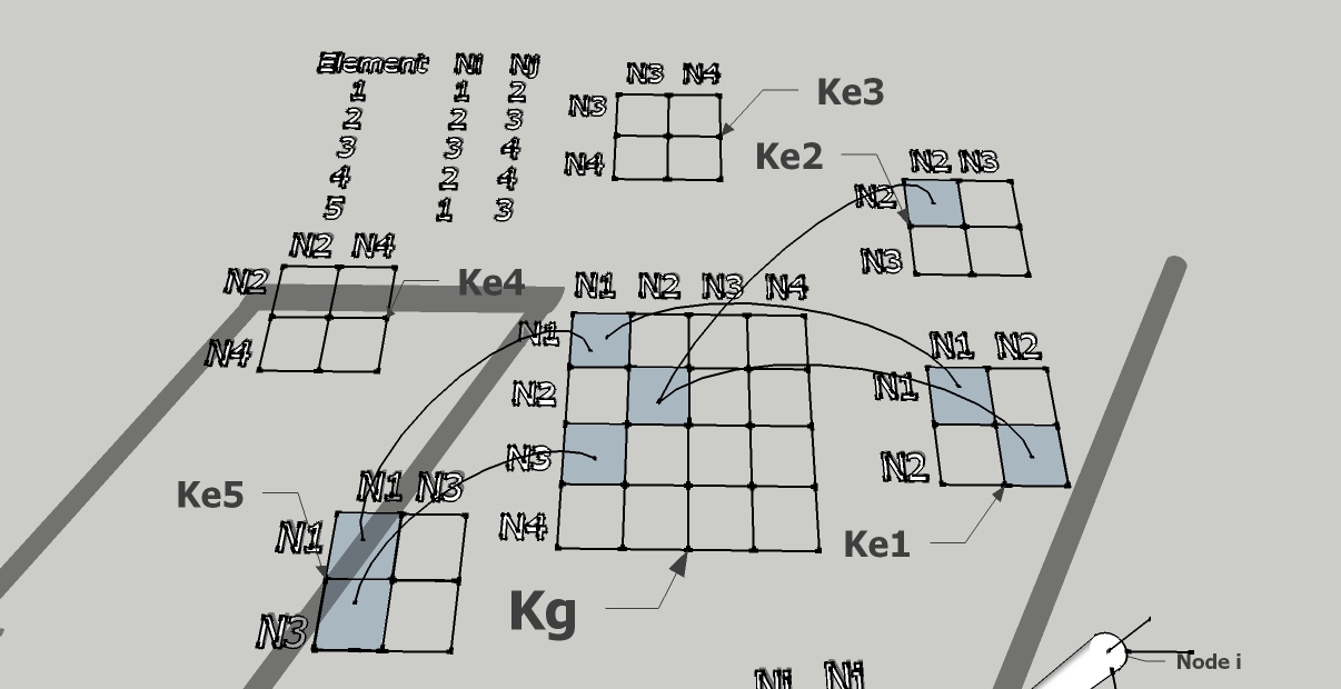
In this basic yet classic example, I have chosen to divide my sample structure in only 5 elements where nodes are clearly identifiable in the meetings between beams. There are four nodes.
 |
| Degrees of Freedom |
Each node will have 6DOF (Degrees Of Freedom): three for linear displacement on each axis (X,Y,Z) and three for rotational around each axis (X,Y,Z), because we are working on 3D. Many examples available provide the more "simple" 2D situation, but in my opinion this only complicates things further.
 |
| A sample structure (mesh) and its topology table |
Once the nodes are located and there is a network of how they relate to each other, we can consider we have a mesh. In our example, the correlation is depicted in the table: The elements serve to "link" nodes to each other. The table establishes a "topology" for the nodes.
STEP 2: Element characterization and shape functions
In this step is where FEM formulation and literature get really really awkward and nasty. In fact, this is the core of everything and where FEM differenciates from other ways of solving PDEs.
 |
| Different types of Finite Elements |
In reality, and despite its mathematical complexity (also unneccesary to be explained so much in detail in my opinion), what we are looking for is a way of characterizing the material properties of the element. For such purpose, the method requires that the behavior of those links among nodes obeys some formula. This formula is the actual
Shape Function. In fact, the shape function can be any mathematical formula that helps us to interpolate what happens wherever there are no points to define the mesh. This "ghost" entity that appears between nodes is in fact the
Finite Element.
In practical terms, as engineers we are more interested in the implementation of the FEM, not so much on its formulation, so what is important to understand is that for different shape functions we obtain different element matrices.
 |
| 2DOF Beam element matrix |
 |
| 3DOF Beam Element matrix |
 |
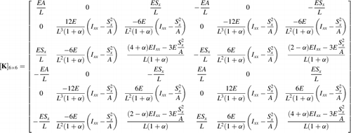
3DOF Timoshenko Beam element matrix
6DOF Timoshenko Beam element matrix |
Depending on the chosen formulation we have different degrees of interpolation and hence presumably higher or lower degrees of precision. Also depending on the chosen formulation we might have different ways of locating and relating our nodes to each other.
For our example we can choose any of the formulations provided in literature (above are the most common used in structural engineering). It is important to note the internal structure of these element matrices, which are symmetrical and clearly divided into parts each corresponding to the nodes that reside on the element's boundaries (2 nodes in the case of a beam - 4 quadrants in the matrix).
STEP 3: Matrix assembly and solution
Because the relations between nodes need to be accomplished all at the same time, we have to set all the equations in such a manner that they compose an algebraic system of equations. The matrix equation we want to solve (at least in statics) is as follows:
[F]= [Kg]·[u]
Where [F] is the vector of applied external forces, [Kg] is the system's global stiffness matrix and [u] is the vector of displacements resulting from the application of the forces. The size of [Kg], [F] and [u] is that of the number of DOFs times the number of nodes, being [Kg] squared and [F] and [u] unidimensional.
In order to generate the Force vector, all we need to do is collect the applied forces (linear and moment forces) and sort them according to the index of the node they are applied to.
For the global stiffness matrix, it is necessary a bit more laborious procedure by means of which we iterate throughout each element's particular stiffness matrix. Out of each one of those, we get only the part that corresponds to the position of the node we are storing in the matrix, and add it to the possible concurrent data that comes from other elements. Warning: before entering in the global stiffness matrix, we must convert local coordinates to global coordinates!
To get the displacement vector, it is needed to first enforce the constraints and then solve the resulting algebraic system of equations. To do this there are two classical approaches: Penalty Method and Lagrange Multipliers method, but we wont enter into this here...
 |
| Global Matrix Assembly |
Afterwards, all we need to do is use any available algebraic equation solver (LU decomposition is one of the most extended), and obtain the solution of the system.